Posts Tagged ‘sql’

Full-text search with PostgreSQL

I spent some time experimenting with PostgresSQL’s full-text search functionality, which has been available to some degree since v8.3. If Postgres is already being used as a data store, this functionality is attractive as it provides a simple way to implement non-trivial search without the need to build out additional infrastructure and code (e.g. an Elasticsearch cluster + application code to load data into Elasticsearch and keep it up-to-date).

I experimented with basic querying and ranking using the Lexiio database, the definitions table in particular provides a good dataset to work with, containing 604,076 term definitions.

Querying

Below is a sample query where we search for the phrase “to break into small pieces”, rank each item in the result set, and order the results based on their rank.

SELECT id, definition
FROM definitions
WHERE to_tsvector('english', definition) @@ plainto_tsquery('english', 'to break into small pieces')

Understanding this query is mostly about understanding some vendor-specific SQL.

  • The tsvector type represents is a sorted list of lexemes. to_tsvector(…) is a function to convert raw text to a tsvector.
  • The tsquery type represents lexemes to be searched for and the operators combining them. to_tsquery(…) is a function to convert raw text to a tsquery.
  • @@ is the match operator, this is a binary operator which take a tsvector and a tsquery

PostgreSQL full-text search query

To get a better understanding of of these types, it can be helpful to run the conversion functions with a few phrases.

SELECT to_tsvector('english', 'to break into small pieces');

"'break':2 'piec':5 'small':4"
SELECT plainto_tsquery('english', 'to break into small pieces');

"'break' & 'small' & 'piec'"

Ranking

The ranking of a full-text search match can be computed with either ts_rank(…), which provides a standard ranking, or ts_rank_cd(…), which gives a coverage density ranking (where ranking is also based on term proximity and cooccurrence, as described in “Relevance ranking for one to three term queries”).

SELECT
id,
definition,
ts_rank(
to_tsvector('english', definition),
plainto_tsquery('english', 'to break into small pieces')
)
AS rank
FROM definitions
WHERE to_tsvector('english', definition) @@ plainto_tsquery('english', 'to break into small pieces')
ORDER BY rank DESC

Higher rank values correspond to more relevant search results.

Here’s the result set, with rankings, for the query above:

+--------+-----------------------------------------------------------------------------------------------------------------------------------------------------------------+----------+ | id | definition | rank | +--------+-----------------------------------------------------------------------------------------------------------------------------------------------------------------+----------+ | 568352 | # {{transitive}} To [[break]] small pieces from. | 0.26833 | +--------+-----------------------------------------------------------------------------------------------------------------------------------------------------------------+----------+ | 135231 | # Resistant to chipping (breaking into small pieces). | 0.266913 | +--------+-----------------------------------------------------------------------------------------------------------------------------------------------------------------+----------+ | 572891 | # {{transitive}} To break into small pieces or fragments. | 0.266913 | +--------+-----------------------------------------------------------------------------------------------------------------------------------------------------------------+----------+ | 568348 | # {{transitive}} To [[break]] into small pieces. | 0.266913 | +--------+-----------------------------------------------------------------------------------------------------------------------------------------------------------------+----------+ | 176962 | # To break into crumbs or small pieces with the fingers; to [[crumble]]. | 0.25948 | +--------+-----------------------------------------------------------------------------------------------------------------------------------------------------------------+----------+ | 50744 | # A small piece of [[detailing]] added to break up the [[surface]] of an [[object]] and add [[visual]] interest, particularly in [[movie]] [[special effect]]s. | 0.25134 | +--------+-----------------------------------------------------------------------------------------------------------------------------------------------------------------+----------+ | 568350 | # {{transitive}} To [[break]] open or [[crush]] to small pieces by impact or stress. | 0.25134 | +--------+-----------------------------------------------------------------------------------------------------------------------------------------------------------------+----------+ | 572890 | # {{transitive}} To break into [[fragment]]s or small pieces. | 0.25134 | +--------+-----------------------------------------------------------------------------------------------------------------------------------------------------------------+----------+ | 547405 | # {{surgery}} The [[operation]] of breaking a [[stone]] in the [[bladder]] into small pieces capable of being [[void]]ed. | 0.221355 | +--------+-----------------------------------------------------------------------------------------------------------------------------------------------------------------+----------+

Indexing

Without an index the above query takes ~5.3 seconds on my local machine (i7-4790K @ 3.7GHz, Intel 730 Series SSD, DDR3 1600 RAM w/ more than enough available to PG).

A Generalized Inverted Index (GIN) is recommended for full-text search. A GIN index can be created directly on a tsvector column or, in this case where there’s an existing text column, an expression index can be created using the to_tsvector() function.

CREATE INDEX ix_def
ON definitions
USING GIN(to_tsvector('english', definition));

With this index, performance improves drastically, with query times ~13 milliseconds.

Is it worth trying?

Maybe. If you’re not using Postgres as the data store for what needs to be searched over (i.e. you’d have to continually ETL data into Postgres), you already have a sophisticated search solution in place, or you’re operating at a scale where you need a clustered solution, probably not. However, if you’re using Postgres, and looking to implement search in an application or move beyond simple substring search, what Postgres is offering is fairly powerful and worth trying out.
Numbering items within groups in MySQL

In my previous post, I described computing row numbers for items within a result set. If items in the result set can be ordered into groups, you can use the same technique to number items within the groups. This is valuable as it allows you to get the top 3, top 5, top N … items within each group (note that GROUP BY isn’t appropriate here; we don’t want to aggregate items within a group, we want an ordering of all the items within a group).

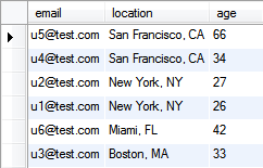
Consider the following sample of data where we’ve done an ordering by the location and age fields (ORDER BY location DESC, age DESC). Every user’s email address is within a group (location) and within that group users are sorted by age in descending order.

SELECT mytable.*
FROM mytable
ORDER BY location DESC, age DESC

ordered data

By using two variables, one to keep track of the item number (@itm) and another to keep track of the current group (@grp), and incrementing the item number if the current group has not changed, else resetting it to 1, we get a numbering of each item within each group. In this example, the group item number tells us who is the 1st oldest, 2nd oldest, etc. user in each location.

SELECT

    
@itm := IF(@grp = location, @itm + 1, 1) AS group_item_number,
    
@grp := location,

    
mytable.*

FROM     mytable,
        (
SELECT @itm := 0) AS itm_num_init,
        (
SELECT @grp := NULL) AS grp_init

ORDER BY location DESC, age DESC

group item numbers

Row numbers in MySQL

Surprisingly straight-forward. Row numbers are useful is cases where you need the rank of a row within a result set.

SET @cur_row := 0;
SELECT mytable.*,
@cur_row := @cur_row + 1 AS row_num
FROM mytable
ORDER BY whatever;

The variable initialization can be done without a SET declaration by doing it as a JOIN:

SELECT mytable.*,
@cur_row := @cur_row + 1 AS row_num
FROM mytable, (SELECT @cur_row := 0) AS row_num_init
ORDER BY whatever;

Solution via Daniel Vassallo’s answer on StackOverflow. A comment mentioned the row numbers being calculated before ordering is done, but I haven’t found this to be the case.

While the above queries will give you the row numbers as expected, putting a HAVING or GROUP BY clause in the same statement might be dangerous. From Xaprb:

The result of assigning to a variable and using it in the same statement (in the HAVING, for example) depends on the query plan the server chooses, the phase of the moon, and probably other things too.

So, in such cases, a subquery is the safe bet:

SELECT sub.* FROM

    
(SELECT mytable.*,
            
@cur_row := @cur_row + 1 AS row_num
    
FROM mytable, (SELECT @cur_row := 0) AS row_num_init
    
ORDER BY whatever) AS sub

HAVING sub.row_num ... ;

Generating a random timestamp in MySQL

Random timestamps are fairly simple to generate and useful when creating test data or fake data for demos. The technique involves converting a MySQL timestamp into unix time, adding or subtracting a certain time range (in seconds), then converting back to a MySQL timestamp.

I’ve used this technique presented on underdog-projects.net before, where a starting timestamp is specified and a random time span is added to the timestamp. However, I wanted to try something slightly different and, in my opinion, a bit more robust. Instead of specifying a starting timestamp, I wanted a pivot timestamp from which a random time span is randomly added or subtracted.

SET @pivot_ts = '2013-01-15 22:15:45';
SET @max_span = 432000; /* 5 days in seconds */
SET @bias = SIGN(-0.5 + RAND());

SELECT FROM_UNIXTIME(
    
UNIX_TIMESTAMP(@pivot_ts) + ( @bias * (FLOOR(RAND()*@max_span)) )
);

Of course all the variables can be made part of the SELECT statement to make everything more succient.

Imperative vs. Declarative Languages

Interesting read. However,

Declar­a­tive lan­guages allows for greater exten­si­bil­ity, agility and pro­duc­tiv­ity.

I don’t know that I would attribute any of these terms to SQL.

NYC Data Mine, restaurant inspection data

I’ve just finished importing the current restaurant inspection data from the NYC Data Mine into a PostgreSQL database. It wasn’t the most difficult migration, but more difficult than it should be as the raw data from the data mine is messy and not well-formed; a typical problem with many of the data sets present in NYC Data Mine. I came across a great post by Steven Romalewski (director of the CUNY Mapping Service) about the poor data quality and poor metadata based on his experiences.

From looking at the restaurant inspection data and skimming a few other sets, I get the sense that structured and relational data simply isn’t understood or handled well. To be fair, there’s a very real lack of tools in the market, at least at the consumer/data-entry level, for handling such data, so it’s not surprising that everything gets jerryrigged into an Excel worksheet. This is very clear when looking at the restaurant inspection data, you notice right away that restaurant ids and names are repeated across multiple rows.

In any case, the restaurant inspection data is better than most of the sets, but there’s a few issues to take note of:

  • In multiple cases the same row, with the exact same data, is repeated.
  • There are 2 columns for the inspection date: INSPDATE and GRADEDATE; GRADEDATE = INSPDATE if there’s a letter grade for the restaurant, otherwise it’s blank/null.
  • Most glaring, there are invalid timestamps in the GRADEDATE column for 2 restaurants (but, of course, it’s across multiple rows as the restaurants has multiple entries), CAPRI RESTAURANT and MAMA LUCIA:

    timestamp problem

For my purposes, I only wanted the most recent inspection result (i.e. the row the latest INSPDATE timestamp). To do this, I added an additional column for a serial/auto_increment id number. Then, once imported, I deleted the unneeded rows with the following query:

/* table is restaurant
id = CAMIS
inspection_score_date = INSPDATE
internal_id = serial/auto_increment id number
*/

DELETE FROM restaurant WHERE internal_id NOT IN
(SELECT MAX(restaurant.internal_id) AS max_iid FROM restaurant,
(SELECT id, dba, MAX(inspection_score_date) AS last_inspt FROM restaurant GROUP BY id, dba) AS sub
WHERE restaurant.id=sub.id AND restaurant.inspection_score_date=sub.last_inspt GROUP BY restaurant.id)

The innermost subquery pulls the rows with the most recent inspection date, the outer takes care of duplicate rows with the same inspection date by simple taking the row with the max internal id number. What results is a column of internal id numbers – each representing a row with a unique restaurant inspection for the most-recent inspection.

I’m not sure if this is the best or most efficient way to do this, but it works and took about 14s to delete the unneeded rows for 398,878 rows on a low-end VPS.