semi/signal

How to local dev

Local developer environments can take many forms but for non-trivial web applications I’m still fond of Vagrant to spin up a VM that is “close enough” to production environments. Typically, I will create a Vagrant box and map a hostname to the IP of the box via an entry in the host system’s hosts file (I use vagrant-hostmap for this, as DHCP is used to avoid conflicts and that means the IP address change often).

Does HTTPS matter for local dev?

Probably not. I went down this particular rabbit hole as I was doing some experiments with server-side events and noticed there’s a limitation on open connection when not using HTTP/2.

So, I thought it would be a good idea to get HTTP/2 working in my local dev environment, which was using Apache and PHP. This is fairly straightforward to setup on Apache. However, the browser (Chrome) was not happy with. Currently, browsers only support HTTP/2 over TLS (h2) and there’s is no support for HTTP/2 Cleartext (h2c). There some good reasons for this.. but many of these reasons are addressing concerns on the public web, for other use-cases (e.g. local dev) there’s additional complexity to support h2 with minimal benefits.

Scripting

The code in the sections below is Bash for a provisioning script (bootstrap.sh), intended to run when the Vagrant is provisioned. The code is such that the environment of the box is reproducible (after destroying and re-creating) and there is no need to re-adjust configuration on the host machine (comes into play when dealing with certificates).

The Vagrantfile looks something like this:

$startScript = <<START_SCRIPT sudo service apache2 restart START_SCRIPT Vagrant.configure("2") do |config| config.vm.box = "ubuntu/mantic64" config.vm.provision :shell, path: "localdev/bootstrap.sh" config.vm.provision "shell", inline: $startScript, run: "always" config.vm.network "private_network", type: "dhcp" end

… with the bootstrap script and related assets (e.g. Apache conf files) within the localdev folder.

Supporting h2: disable prefork

First, disable the prefork module, it doesn’t play well with HTTP/2:

sudo a2dismod mpm_prefork

In prefork, mod_http2 will only process one request at at time per connection. But clients, such as browsers, will send many requests at the same time. If one of these takes long to process (or is a long polling one), the other requests will stall.

Supporting h2: enable HTTP/2 modules and configuration

Enable modules and configuration for HTTP/2:

sudo a2enmod mpm_event sudo a2enmod http2 sudo cp /vagrant/localdev/http2.conf /etc/apache2/conf-available/http2.conf sudo a2enconf http2

The http2.conf file contains the following:

<IfModule http2_module> Protocols h2 h2c http/1.1 H2Direct on </IfModule>

Required modules and configuration are now enabled. For a given VirtualHost definition, you can add Protocols h2 h2c http/1.1.

e.g.:

<VirtualHost *:443> ServerAdmin webmaster@localhost DocumentRoot /var/www/html Protocols h2 h2c http/1.1 ...

Supporting h2: minica

For HTTPS TLS certificate generation, minica is awesome and simple to use. However, it is only distributed as source, so you’ll need to install git to checkout the repo and golang to compile the source.

sudo apt-get -y install git sudo apt-get -y install golang-go sudo mkdir /certs sudo mkdir /tools cd /tools git clone https://github.com/jsha/minica.git cd /tools/minica go env -w GO111MODULE=auto go build -buildvcs=false

Here a /tools folder is created, the minica repo is cloned within, and the source is compiled.

A /certs folder is also created as a location for generated certificates.

Supporting h2: generate root CA certificate

Once compiled, run minica to generate a root CA certificate (minica.pem) and key (minica-key.pem), which can be installed on the host to avoid browsers showing that the certificate is invalid or untrusted. This shouldn’t be done in the Vagrant box provisioning script, as you’ll get new root certificates every time the box is provisioned. Instead, SSH into the box, run, and copy the files to a secure location.. or run minica somewhere else (e.g. host machine or another machine). ./minica --domains "test.localdev.com"

minica requires a domain argument but the need is really for the minica.pem and minica-key.pem files at this point, not the site certificate. Generation of the site certificate is something that should be done within the provisioning script.

Supporting h2: generate site certificate

Within the provisioning script:

SITE_DOMAIN="localdev.com" WILDCARD_CERT="*.localdev.com" CERT_FOLDER="_.$SITE_DOMAIN"; CA_CERT="/vagrant/localdev/secrets/minica.pem" CA_KEY="/vagrant/localdev/secrets/minica-key.pem" ./minica --ca-cert "$CA_CERT" --ca-key "$CA_KEY" --domains "$WILDCARD_CERT" cp -R "/tools/minica/$CERT_FOLDER" "/certs/$CERT_FOLDER"

There’s a 2 things to note here:

• To avoid having to generate new certificates for different subdomains, a wildcard cert is generated (*.localdev.com)
• An existing root CA certificate, and key, is expected

Supporting h2: use site certificate

Update the VirtualHost definition to reference the site certificate and key:

<VirtualHost *:443> ServerAdmin webmaster@localhost DocumentRoot /var/www/html Protocols h2 h2c http/1.1 SSLEngine on SSLCertificateFile /certs/_.localdev.com/cert.pem SSLCertificateKeyFile /certs/_.localdev.com/key.pem ...

Trusting minica certs on the host

Finally, to avoid the browser showing a warning that the site’s certificate is invalid or insecure, add the root certificate as a trusted root CA authority on the host machine. Martin Widmann has some nice documentation on how to do this for different operating systems.

Verify h2 protocol in the browser

With the site up, Chrome and Firefox dev tools should now show that traffic is being served via the h2 protocol.

The Protocol column isn’t visible by default, so you may have to enable it (right click on visible header → select Protocol).

Something I read a long time ago that comes to mind when I think about engineering team culture is this interview around design at Apple. Specifically, the myth around Apple having the best designers:

I think the biggest misconception is this belief that the reason Apple products turn out to be designed better, and have a better user experience, or are sexier, or whatever … is that they have the best design team in the world, or the best process in the world…

It’s actually the engineering culture, and the way the organization is structured to appreciate and support design. Everybody there is thinking about UX and design, not just the designers. And that’s what makes everything about the product so much better … much more than any individual designer or design team.

[Aside: looking back a bit, it’s worth noting that, more-so in 2014 than now, Apple’s products were viewed as being far superior in design to competitors. Many people I worked with pointed to how something looked or functioned on a Mac or iPhone as the ideal and there was a desire to replicate that aesthetic and experience. Now, in 2024, Apple is still known for good design, but I don’t think they have the same monopoly that they did a decade ago.]

What resonates here is how the concern (for a better user experience, better product, etc.) needs to be embedded within the culture of the team and it’s not something can be be strictly delegated to a certain individual, role or team (and then “thrown over the wall”).

Of course this is maybe not too surprising, within software engineering itself there’s been a need/desire/push to diffuse concerns around operations, security, testing, etc. (and what actually got me thinking about this was actually the interplay between application engineers and security engineers, where application engineers can’t simply “hand off” security concerns).

A few months ago, being particularly frustrated by yet-another-bug and yet-another-limitation of a library used in one of my team’s systems, I remembered a story about the Excel dev team and dug up In Defense of Not-Invented-Here Syndrome, which I read years ago. I didn’t think much of the essay when I first read it but now, having been in the industry for a while, I have a greater appreciation for it.

NIH syndrome is generally looked at in a negative light and for good reason; companies and teams that are too insular and reject ideas or technologies from the outside can find themselves behind the curve. However, there’s a spectrum here and, at the opposite end, heedless adoption of things from the outside can put companies and teams in an equally precarious position.

So, back to the story of the Excel development team:

“The Excel development team will never accept it,” he said. “You know their motto? ‘Find the dependencies — and eliminate them.’ They’ll never go for something with so many dependencies.”

Dealing with dependencies is a reality of software engineering, perhaps even more-so now than in the past, and for good reason, there’s a world of functionality that can simply be plugged into a project, saving significant amounts of time and energy. However, there’s a number of downsides as well:

• Your team doesn’t control control the evolution or lifecycle of that dependency
• Your team doesn’t control the quality of that that dependency
• Your team doesn’t have knowledge of how that dependency does what it does

When something breaks or you hit a limitation, your team is suddenly spending a ton of time trying to debug an issue that originates from a codebase they’re not familiar with and, once there’s an understanding of the issue, coding some ugly hack to get the dependency to behave in a more reasonable way. So when a team has the resources it’s not unreasonable to target elimination of dependencies for:

• A healthier codebase
• A codebase that is more easily understood and can be reasoned about

These 2 points invariably lead to a higher performing team. In the case of the Excel dev team:

The Excel team’s ruggedly independent mentality also meant that they always shipped on time, their code was of uniformly high quality, and they had a compiler which, back in the 1980s, generated pcode and could therefore run unmodified on Macintosh’s 68000 chip as well as Intel PCs.

Finally, Joel’s recommendation on what shouldn’t be a dependency and be done in-house:

Pick your core business competencies and goals, and do those in house.

This makes sense and resonates with me. Though there is a subtle requirement here that I’ve seen overlooked: engineering departments and teams need to distill business competencies and goals (hopefully, these exist and are sensible) into technical competencies and goals. Without that distillation, engineering is rudderless; teams pull in dependencies for things that should be built internally, while others sink time into building things from scratch that will never get the business resources to be properly developed or maintained.

The observers

MutationObserver, along with its siblings ResizeObserver and IntersectionObserver, are great tools for working with the DOM. I don’t think there’s necessarily broad usage of these observers in frontend development but, when building applications that need insight into lower-level DOM changes, they are powerful interfaces and allow you to avoid the typical/hacky solution of polling for changes.

Interface

All the observer classes share a common, fairly simple interface. There’s just a few key aspects needed to use them:

• The constructor takes a callback, which is called whenever the DOM state change corresponding to the class (mutation, resize, etc.) is observed.
• The observe() method takes a target DOM element to observer

On an observed state change (e.g. mutation) the given callback is called with an appropriate record (e.g. MutationRecord)

Missing context

The records surfaced on an observed state change contain information about the change but nothing around who or what triggered the change. Looking at a comparable scenario, this is typically the case for most DOM events as well, but it’s generally a non-issue because you can reasonably assume that the event was triggered by the user interacting with the browser. When it comes to changes detected by an observer, there’s a bit more ambiguity as to how the change came about and you can’t always assume the change was from the end-user.

Note: yes, you an programmatically force DOM events to be emitted as well (e.g. element.click()) but I think this is almost always an anti-pattern

For example, let’s say you have an application where you allow users to enter content into a contenteditable <div> but you’d also programmatically surface and incorporate content coming from the server (from other internet users using the application). Ideally, you could use a MutationObserver on the <div> to detect changes and see if there’s new content that needs to be sent to the server, but you’d need to distinguish:

• What changes are coming from the user interacting with the browser
• What changes are being made programmatically (i.e. coming from other server / coming from other users)

Unfortunately, you can’t make this distinction with the information surfaced in a MutationRecord.

While DOM events don’t necessarily map to an actor model, I tend to think what’s conceptually missing here is knowing the originating actor of the events/message and, in any user-facing system, there’s going to be at least 2 actors:

• The system
• The end-user interacting with the system

Once you’re within a system dealing with mutating state, knowing who the originating actor is incredibly valuable information.

Hacking around this

I’m prototyping a hacky, but reasonable, solution for ScratchGraph:

Overall, this seems to work but I hate patterns like this where I have to purposely introduce latency.

Whitespace and tags

Previously, I looked at improving the functionality of strip_tags such that words across tags are not mashed together. The method I derived works well enough but it’s limited in that all tags are treated the same way and all whitespace separators are the same. I wanted to see if I could improve the method a bit more to address these limitations; that is, introducing whitespace based on the type of tag encountered instead of injecting whitespace after stripping away a tag.

For example, when dealing with inline tags, whitespace should be preserved:

This bit of HTML:

<span>the quick brown fox </span><span>jumped over the moon</span>

… should produce:

the quick brown fox jumped over the moon

Alternatively, when dealing with block-level tags, a newline should be injected:

This bit of HTML:

<div>the quick brown fox</div><div>jumped over the moon</div>

… should produce:

the quick brown fox jumped over the moon

Note that we’re simply talking about common/expected browser behavior from what’s thought of as inline-level or block-level tags. In reality, this categorization isn’t really part of the HTML standard anymore and layout behavior is relegated determined by CSS. From MDN:

That said, when looking at arbitrary HTML content, I still think “block” vs. “inline” is a useful distinction, at least insofar as inferring default or common behavior.

The special case

The <br> tag presents a special case. While it’s classified as an inline element, <br> represents whitespace that is generally similar to that of a block-level element (e.g. a newline). In implementation this is simple to handle but does introduce a tiny bit of additional complexity.

Looking at the high-level transformations needed, we get the following:

• Inline-level tags → strip away (no action needed, don’t alter any existing whitespace within tag contents)
• Block-level tags → strip away, replace with newline
• <br> tags → strip away, replace with newline

Code

Reworking the convert() method from the previous post, we get the following:

class HTMLToPlainText { const BLOCK_LEVEL_ELEMENTS = [ "address", "article", "aside", "blockquote", "details", "dialog", "dd", "div", "dl", "dt", "fieldset", "figcaption", "figure", "footer", "form", "h1", "h2", "h3", "h4", "h5", "h6", "header", "hgroup", "hr", "li", "main", "nav", "ol", "p", "pre", "section", "table", "ul" ]; const INLINE_LEVEL_ELEMENTS_THAT_PRODUCE_NEWLINE = [ "br", ]; const STATE_READING_CONTENT = 1; const STATE_READING_TAG_NAME = 2; static public function convert(string $input, string $blockContentSeparator = "\n"): string { // the input string as UTF-32 $fixedWidthString = iconv('UTF-8', 'UTF-32', $input); // string within tags that we've found $output = ""; // buffer for current/last tag name read $currentTagName = ""; $currentTagIsClosing = null; // buffer content in the current tag being read $contentInCurrentTag = ""; // flag to indicate how we should interpret what we're reading from $fixedWidthString // .. this is initially set to STATE_READING_CONTENT, as we assume we're reading content from the start, even // if we haven't encountered a tag (e.g. string that doesn't contain tags) $parserState = self::STATE_READING_CONTENT; $flushCurrentToOutput = function() use (&$output, &$contentInCurrentTag, &$currentTagName, &$currentTagIsClosing, &$blockContentSeparator) { // handle inline tags, which produce a newline (e.g. <br>) // .. not that these can be empty (<br>) or self-closing (<br/>) if(in_array(strtolower($currentTagName), self::INLINE_LEVEL_ELEMENTS_THAT_PRODUCE_NEWLINE)) { $output .= $contentInCurrentTag . $blockContentSeparator; } else { // append $blockContentSeparator if we're at the *opening or closing* of a block-level element // (for inline element, leave content as-is) if (in_array(strtolower($currentTagName), self::BLOCK_LEVEL_ELEMENTS)) { $output .= $contentInCurrentTag . $blockContentSeparator; } else { $output .= $contentInCurrentTag; } } // reset $contentInCurrentTag = ""; $currentTagIsClosing = null; $currentTagName = ""; }; // iterate through characters in $fixedWidthString // checking for tokens indicating if we're within a tag or within content for($i=0; $i<strlen($fixedWidthString); $i+=4) { // convert back to UTF-8 to simplify character/token checking $ch = iconv('UTF-32', 'UTF-8', substr($fixedWidthString, $i, 4)); if($ch === '<') { $flushCurrentToOutput(); $parserState = self::STATE_READING_TAG_NAME; continue; } if($ch === '>') { $flushCurrentToOutput(); $parserState = self::STATE_READING_CONTENT; continue; } if($parserState == self::STATE_READING_TAG_NAME && $ch == '/') { $currentTagIsClosing = true; continue; } if($parserState == self::STATE_READING_TAG_NAME) { $currentTagName .= $ch; continue; } if($parserState === self::STATE_READING_CONTENT) { $contentInCurrentTag .= $ch; continue; } } $flushCurrentToOutput(); return trim($output, $blockContentSeparator); } }

Testing

Throwing some arbitrary bits of HTML at this function seems to indicate that the method works correctly but, a method like this, really calls for some form of automated testing. I could derive test cases from the function logic, and this is what’s typically done when testing some arbitrary method, but this approach is biased and limited here. Biased in that I’d be looking at the function and coming up with test cases based upon my experiences (what I’ve encountered and where I think there may be potential issues). Limited in that I’d likely only come up with a handful of test cases unless I invested a significant chunk of time into compiling a comprehensive set of cases; HTML has relatively few building blocks but, given the number of different ways those blocks can be combined and arranged, we end up with a fairly large number of permutations. What would really be effective here is testing with a large and varied corpus of test cases, mappings of HTML snippets to plain text representations; i.e. data-driven testing. It’s usually hard to generate or find data for such testing but the PHP repository has a number of test cases for strip_tags() that can be leveraged:

• strip_tags_basic1.phpt has some good baseline tests (HTML tags, PHP tags, tags with attributes, HTML comments, etc.)
• strip_tags_basic2.phpt has a good test case (different tags + mix of block and inline elements + PHP tags) but is really testing the allowed_tags_array argument to strip_tags(), which I forgot was a thing and didn’t consider in my method

Beyond the test cases in these 2 files, there are other good cases scattered in the repo, seemingly tied to specific bugs encountered (e.g. bug #53319, which involves handling of “<br />” tags) but they can be hard to locate given the organization or lack thereof of the test files. In any case, it’s great having this data to work with and there were some issues that surfaced when I began subjecting my code to some of these test (e.g. the content separator for block-level elements needing to be attended at the point of both the opening and closing tags, not just the closing tag).

Implementation-wise, testing is mainly encoding the test case in a map and assert that the actual result matches expectations:

$testCases = [ "<html>hello</html>" => "hello", "<?php echo hello ?>" => "", "<? echo hello ?>" => "", "<% echo hello %>" => "", "<script language=\"PHP\"> echo hello </script>" => " echo hello ", "<html><b>hello</b><p>world</p></html>" => "hello\nworld", "<html><!-- COMMENT --></html>" => "", "<html><p>hello</p><b>world</b><a href=\"#fragment\">Other text</a></html><?php echo hello ?>" => "hello\nworldOther text", "<p>hello</p><p>world</p>" => "hello\n\nworld", '<br /><br />USD<input type="text"/><br/>CDN<br><input type="text" />' => "USD\nCDN", ]; foreach ($testCases as $html => $expectedPlainText) { $actualPlainText = HTMLToSearchableText::convert_ex($html); echo "TEST: " . $html . "\n"; echo "EXPECTED: " . $expectedPlainText . "\n"; echo "ACTUAL: " . $actualPlainText . "\n"; echo "----\n"; assert($actualPlainText === $expectedPlainText); }

Testing is still limited here. I’ve love to simply have a large batch of test cases to throw at the function but something like that is not readily available.

Limitations / future work

The new convert() method is more robust but there’s still some key limitations when compared to the strip_tags() function:

• PHP’s strip_tags() is actually a lot more robust when it comes to invalid/malformed HTML content, as the tests in strip_tags.phpt demonstrate
• Preserving certain tags (as with the allowed_tags_array argument) wasn’t considered

Also, whitespace/separators produced from <br> elements at the beginning or end of any inputted HTML is stripped away. I don’t think this is correct as browsers preserve whitespace from <br> elements and don’t collapse them as with empty block-level elements.

I did some quick benchmarking with canvas-image-transformer, looking at the performance between directly manipulating pixels on a 2D canvas versus using a fragment shader on a WebGL canvas. For testing, I used a grayscale transformation as it can be done with a simple weighted sum (R*0.2126 + G*0.7152 + B*0.0722) and there’s a high degree of parity between the fragment shader code and the code for pixel operations on a 2D canvas.

Converting to grayscale

Pixel operations on the 2D canvas are as follows:

for(var i=0; i<pixels.data.length; i+=4) { var grayPixel = parseInt(((0.2126*(pixels.data[i]/255.0)) + (0.7152*(pixels.data[i+1]/255.0)) + (0.0722*(pixels.data[i+2]/255.0))) * 255.0); pixels.data[i] = grayPixel; pixels.data[i + 1] = grayPixel; pixels.data[i + 2] = grayPixel; }

The corresponding fragment shader for the WebGL canvas is as follows:

precision mediump float; uniform sampler2D uSampler; varying vec2 vTextureCoord; void main(void) { vec4 src = texture2D( uSampler, ( vTextureCoord ) ); float grayPx = src.r*0.2126 + src.g*0.7152 + src.b*0.0722; gl_FragColor = vec4(grayPx, grayPx, grayPx, 1); }

Performance comparisons in Chrome

Here’s the setup for comparing performance of the 2 method:

• Input was a 3864×3864 image of the Crab Nebula, rendered onto a 2D canvas (note that time to render onto the 2D canvas is not considered in the data points below)
• Output is the 2D canvas that the input image was render on
• CPU was an AMD Ryzen 7 5700X
• GPU was a RTX 2060
• OS is Windows 10 Build 19044
• Browser is Chrome 108.0.5359.125
• Hard refresh on page load to bypass any browser-level caching
• Transformation via WebGL approach for 25 iterations
• Transformation via 2D canvas approach for 25 iterations

Visually, this is what’s being done:

I tried to eliminate as much background noise as possible from the result; that is, eliminating anything that may have a impact on CPU or GPU usage: closing other applications that may have significant usage, not having any other tabs open in the browser, and not having DevTools open when image processing was being done. That said, I was not rigorous about this and the numbers presented are to show overall/high-level behavior and performance; they’re not necessarily representative of what peak performance would be on the machine or browser.

It’s also worth noting that canvas-image-transformer doesn’t attempt to do any sort of caching in the first iteration (i.e. textures are re-created, shaders are re-compiled, etc. on each iteration), so we shouldn’t expect large variances in performance from one iteration to the next.

Graphing the data points for each approach, for each iteration, I got the following (note that what’s presented is just the data for 1 test run; I did test multiple times and consistently saw the same behavior but, for simplicity, I just graphed the values from 1 test run):

So, the data points for the first iteration are interesting.

• On the 2d canvas, the transformation initially takes 371.8ms
• On the webgl2, the transformation initially takes 506.5ms

That’s a massive gap in performance between the 2 methods, with the 2d canvas method being significantly faster. I would have expected the WebGL approach to be faster here as, generally, graphics-related things would be faster with a lower-level GPU interface, but that’s clearly not the case here.

For subsequent iterations, we can see that performance improves and normalizes for both approaches, with significantly better performance using the WebGL approach; however, why don’t we see this sort of performance during the first iteration? Profiling the code, I noticed I was consistently seeing the majority of execution time spent on texImage2D() during the first iteration:

gl.texImage2D(gl.TEXTURE_2D, 0, gl.RGBA8, gl.RGBA, gl.UNSIGNED_BYTE, srcCanvas);

Looking at the execution time of texImage2D() across iterations, we get the following:

We see 486.9ms spent in texImage2D() during the first iteration but then execution time drops to only ~0.1ms in subsequent iterations. It’s clear that loading data into a texture is the most costly operation on the first iteration, however it looks like there’s some sort of caching mechanism, likely in Chrome’s GPU component, that essentially eliminates this cost on subsequent iterations.

In an attempt to optimize the call in the first iteration, I briefly looked into potential optimizations to the texImage2D() call but didn’t find much. There’s no mipmap creation or doing any sort of format conversion here, so we’re just bound by how quickly we can get the pixels into VRAM.

Normal refresh (after previous page load)

There’s a bit more nuance here that’s worth touching on. Looking at just the first iteration in Chrome, after normal/soft refreshes, we see some interesting behavior:

• For the 2d canvas, the first iteration transformation times look the same as when doing a hard refresh
• For the WebGL canvas, we’re getting the transformation times we saw after the first iteration when doing a soft refresh!

It looks like Chrome’s texture caching mechanism is in play and preserves cache entries across soft page refreshes.

What about Firefox and other browsers?

I would expect most Webkit-based browsers would have similar behavior to what’s in Chrome and some quick testing in Edge confirms this.

Firefox is a different beast. Testing in Firefox 108.0.2, we see the following transformation times:

Performance, overall, is much more consistent than in Chrome, but not always better.

• For the 2d canvas method, performance is simply worse; on the first iteration we see transformations take 150+ milliseconds more than in Chrome, and on subsequent iterations the performance gap is even wider.
• For the WebGL method, our first iteration performance is significantly better than Chrome, reduced by more than 175 milliseconds. However, on subsequent iterations we don’t see the drastic performance improvement we see in Chrome.

For the 2d canvas method, it’s hard to say why it performs so differently than Chrome. However, for the WebGL method, a bit of profiling led to some interesting insights. In Firefox, the execution time of texImage2D() is consistent across iterations, hovering ~40ms; this means it performs significantly better than Chrome’s worst case (first iteration) and significantly worse than Chrome’s best case (non-first iteration where execution time is below 0.1ms), as shown below.

The other significant aspect to Firefox’s performance is in the performance of the Canvas drawImage() call, in drawing from a WebGL canvas to a 2D canvas. At the tail end of the transformation process, canvas-image-transformer does the following:

const srcCtx = srcCanvas.getContext('2d'); srcCtx.drawImage(glCanvas, 0, 0, srcCanvas.width, srcCanvas.height);

Basically, it’s taking what’s on the WebGL canvas and writing it out to the input/source canvas, which is a 2D canvas. In Chrome this is a very fast operation, typically less that 2ms, in Firefox I see this typically going above 200ms.

Firefox consistency

Finally, looking at transformation times across soft refreshes, we see Firefox performance is very consistent for both the 2D canvas and WebGL method:

However, I did encounter a case where WebGL performance was more erratic. This was testing when I had a lot of tabs open and I suspect there was some contention for GPU resources.

Takeaways

There’s perhaps a number of small insights here depending on use-case and audience, but there’s 2 significant high-level takeaways for me:

• GPUs are very fast at parallel processing but loading data to be processed and retrieving the processed data can be expensive operations
• It’s worthwhile to measure things; I was fairly surprised by the different performance profiles between Firefox and Chrome

Contracts

An issue I’ve kept coming across when working on data systems that involve producing and consuming a number of different datasets is the lack of a contract between producers and consumers. Versioning provides a solution to this problem when dealing with software and, with a decent versioning scheme, provides a good solution for datasets as well, allowing for the creation of versioned snapshots.

Data concerns

It’s worth looking at what the problem is here and why this even matters. Imagine having some dataset, let’s say for drugs, which is periodically updated. We could reasonably say that we only care about the latest version of the drugs dataset, so every time we ingest new data, we simply overwrite the existing dataset.

For a rudimentary system, this is fine, but if we’re thinking in terms of a larger data system with this dataset being consumed by downstream processes, teams, and/or customers, there are a few concerns our system can’t elegantly deal with:

• Corruption: the ingested data is corrupt or a bug in the ETL process results in a corrupted dataset
• Consistent reads: not all parts (e.g. tables) of our dataset may be ready for reads by consumers at a given time (loading data to S3 is a good example here; for a non-trivial dataset with multiple objects and partitions, spread across multiple objects, the dataset as a whole can’t be written/updated atomically)
• Breaking changes: a breaking change to downstream systems (e.g. dropping a column) may need to be rolled out
• Reproducibility: downstream/derived datasets may need to be re-created based upon what the dataset was at some point in the past (i.e. using the latest dataset will not give the same results)
• Traceability: we may need to validate/understand how a derived data element was generated, requiring an accurate snapshot of all input data when the derived dataset was generated

Versioning isn’t the only solution to these concerns. You could argue that frequent backups, some sort of locking mechanism, coordination between teams, and/or very granular levels of observability can address each to varying degrees, but I think versioning is (a) simple and (b) requires the least effort.

Versioning scheme

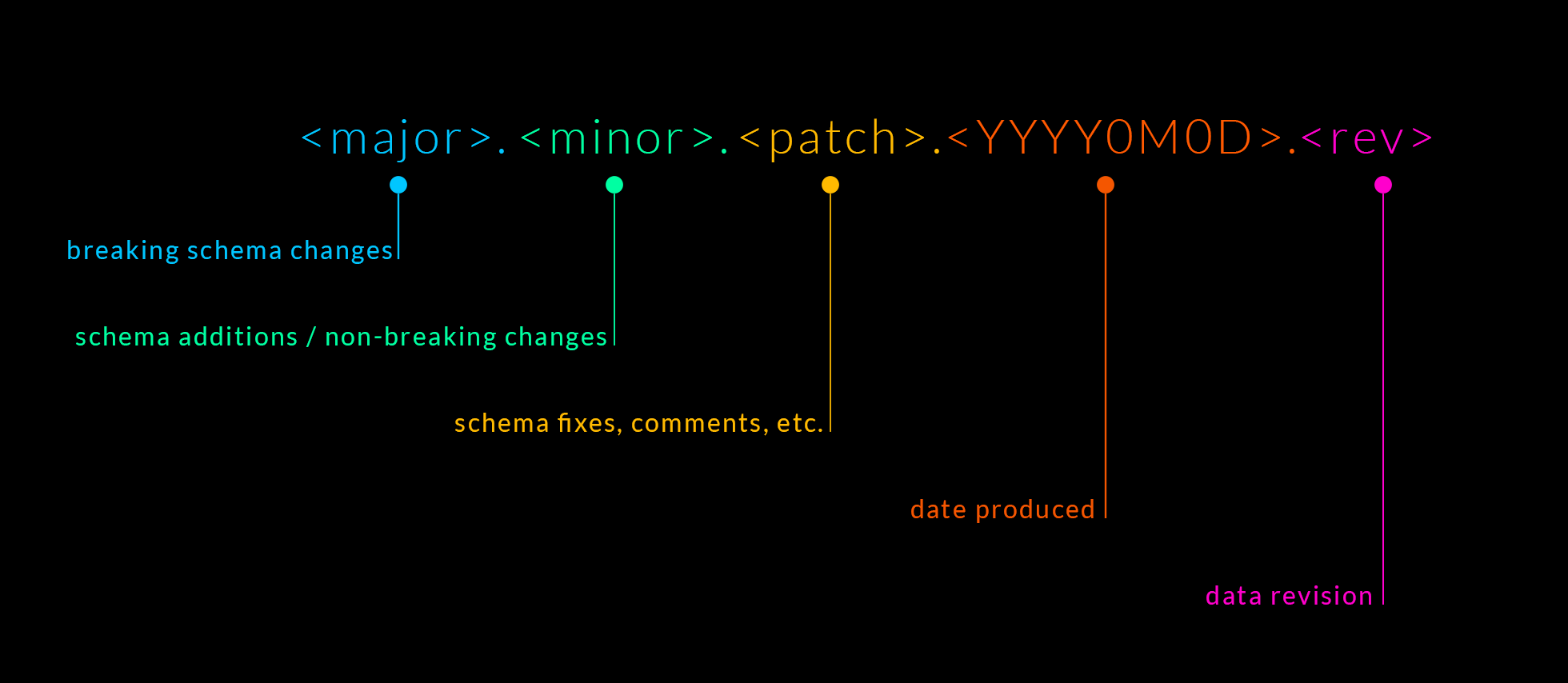
Let’s look at a versioning scheme that would address the 4 concerns I raised above. For this, I’m going to borrow from both semantic versioning and calendar versioning. Combining the 2, and adding a bit of additional metadata, we can construct a scheme like the following:

Breaking this down:

• The semantic versioning components (major, minor, patch) can effectively tell us about the spatial nature of the dataset; the schema.
• The calendar versioning components (YYYY0M0D) can effectively tell us about the temporal nature of the dataset (when it was ingested, generated, etc.). Note that calendar versioning is a lot more fuzzy as a standard, as there’s a lot of variance in how dates are represented, YYYY0M0D seems like a good choice as it’s easily parsable by consumers.
• The final component (rev) is the revision number for the given date and is needed for datasets that can be generated/refreshed multiple times in a day. I think of this as an incrementing integer but a time component (hours, minutes, seconds) is another option; either can work, there’s just tradeoffs in implementation and consumer expectations.

Finding a version

Going back to our example, our data flow now looks something like this:

Note that before our consumers knew exactly where to look for the dataset (s3://bucket/drugs-data/latest), more specifically the latest version of the dataset, however, this is no longer the case. Consumers will need to figure out what version of the dataset they want. This could be trivial (e.g. consumers just want to pin to a specific version) but the more interesting and perhaps more common case, especially with automated systems, is getting the latest version. Unpacking “latest” is important here: consumers want the latest data but not if it carries with it a breaking schema change (i.e. consumers want to pin to major version component, with the others being flexible). Thinking in terms of npm-esque ranges with the caret operator, a consumer could specify a version like ^2.2.11.20221203.1 indicating they system is able to handle, and should pull in, any newer, non-breaking, updates in either schema or data.

So consumers can indicate what they want, but how does a system actually go about finding a certain version? I think the elegant solution here is having some sort of metadata for the dataset that can tell consumers what versions of the dataset are available and where to find them. Creating or updating these metadata entries can simply be another artifact of the ETL process and can be store alongside the dataset (in a manifest file, a table, etc.). Unfortunately, this does involve a small lift and a bit of additional complexity for consumers, as they’d have to read/parse the metadata record.

Dataset-level vs. Data-level versioning

In researching other ways in which versioning is done, change data capture methods usually come up. While change data capture methods are important and powerful, CDC methods are typically at the row-level, not the dataset-level, and it’s worth recognizing the distinction, especially from data systems perspective, as CDC methods come with very different architectural and implementation concerns.

For example, in this blog post from lakeFS, approach #1 references full duplication, which is dataset versioning, but then approach #2 references valid_from and valid_to fields, which is a CDC method and carries with it the requirement to write queries that respect those fields.

Avoiding full duplication

The scheme I’ve laid out somewhat implies a duplication of records for every version of a dataset. I’ve seen a number of articles bring this up as a concern, which can very well be true in a number of case, but I’m skeptical of this being a priority concern for most businesses, given the low cost of storage. In any case, I think storage-layer concerns may impact how you reference versions (more generally, how you read/write metadata), but shouldn’t necessarily dictate the versioning scheme.

From what I’ve read, most systems that try to optimize for storage do so via a git-style model. This is what’s done by cloud service providers like lakeFS and tools like git LFS, ArtiV, and DVC.

Alternatives

I haven’t come across much in terms of alternatives but, in addition to a semantic identifier, this DZone article also mentions data versions potentially containing information about the status of the data (e.g. “incomplete”) or information about what’s changed (e.g. “normalized”). These are interesting ideas but not really something I’ve seen a need for in the version identifier. That said, what I’ve presented is not intended to be some sort of silver bullet, I’m sure different engineers face different concerns and different versioning schemes would be more appropriate.

In the end, I would simply encourage engineers to consider some form of versioning around their datasets, especially in larger data systems. It’s a relatively simple tool that can elegantly address a number of important concerns.

What is S.M.A.R.T.?

Self-Monitoring, Analysis and Reporting Technology (S.M.A.R.T) is a monitoring system on computer hard drives and solid state drives. SMART primarily consists of a set of a attributes, with the disk monitoring current and worst values for said attributes. The attributes, associated ID number, and the range for normalized values (1 to 253) are standardized across disks. Unfortunately, there’s no standardization around which attributes are implemented, the range for raw values, what raw values actually represent, or what the threshold is for normalized value. Despite the lack of standardization around the attribute values, SMART still provides some value and offers a significant degree of observability into the state and behavior of the disk.

SMART is something I’ve been aware of for a while, but it never seemed to really matter all that much for my consumer desktop needs. There are a bunch of Windows apps to check the SMART attributes and I vaguely recall having something installed to check for out-of-range values but regularly monitoring/checking wasn’t something I took seriously; just having a backup was typically good enough and I could deal with a drive failure if/when it happened. Recently, motivated by re-using an old motherboard and CPU for a NAS server, making use of a batch of old hard disks I had accumulated, and maximizing the storage capacity of the box, I decided to take another look at SMART and its efficacy in predicting drive failures. Ideally, I could have a system where a drive could be replaced before a failure resulting in data loss.

SMART attributes correlated to hard drive failure

Google

A Google study from 2007, “Failure Trends in a Large Disk Drive Population“, lists 4 SMART attributes that are highly correlated with failure, these are:

• SMART 5: Reallocated Sectors Count
• SMART 187: Reported Uncorrectable Errors
• SMART 197: Current Pending Sector Count
• SMART 198: Uncorrectable Sector Count

It’s also worth noting that any change in SMART 187 was seen to be highly predictive of failure:

… after their first scan error (i.e. when a positive value for 187 is observed for the first time), drives are 39 times more likely to fail within 60 days than drives with no such errors.

Other attributes were looked at but results were not always consistent across models and manufacturers. The study also found using SMART parameters to predict failure was severely limited, as a large number of failed drives shown no SMART errors whatsoever:

Out of all failed drives, over 56% of them have no count in any of the four strong SMART signals, namely scan errors, reallocation count, offline reallocation, and probational count. In other words, models based only on those signals can never predict more than half of the failed drives.

… even when we add all remaining SMART parameters (except temperature) we still find that over 36% of all failed drives had zero counts on all variables.

… failure prediction models based on SMART parameters alone are likely to be severely limited in their prediction accuracy, given that a large fraction of our failed drives have shown no SMART error signals whatsoever.

This is incredibly important as correlating SMART attributes to failure means little if the correlation simply doesn’t matter for a significant percentage of drives. From skimming a few other papers, this is also something that I don’t always see being addressed/re-addressed, which is disappointing.

Backblaze

Backblaze conducted an analysis on their drives in 2016 which also showed some interesting results. In addition to the 4 SMART attributes identified in the Google study, Backblaze also found another attribute highly correlated to failure:

• SMART 188: Command Timeout

Similar to the Google study, Backblaze also found a significant number of failed drives reporting no SMART errors for these 5 attributes but, interestingly, it was a smaller percentage that that in the Google study:

Failed drives with one or more of our five SMART stats greater than zero: 76.7%.

That means that 23.3% of failed drives showed no warning from the SMART stats we record.

Another study utilizing Backblaze’s data, “Lifespan and Failures of SSDs and HDDs: Similarities, Differences, and Prediction Models“, was also interesting as it points to another attribute highly correlated with failure:

• SMART 240: Head Flying Hours

We examine all SMART features for HDDs, and find out that head flying hours (HFH, SMART 240) is highly related to failures even if it is not correlated with other HDD features.

A more recent post from Backblaze looks at the paper “Interpretable predictive maintenance for hard drives” which utilizes data published from Backblaze. I didn’t have a clear takeaway from the paper it did highlight the limitation of previous studies:

The analyses from Backblaze and Google were univariate and only considered correlation between failures and a single metric at a time. As such, they would not be able to detect any nonlinear interactions between metrics that affected the chance of failure. Another limitation of this analysis is that it leaves humans to choose the cutoff values that will raise alerts if exceeded.

So, for hard drives, SMART is interesting. We can say that there are maybe 6 attributes we should definitely be looking at when observing for drive failure but, unfortunately, a drive may still fail without showing any anomalous values for these attributes.

SMART attributes correlated to solid-state drive failure

While their price-per-gigabyte is still much higher than that of a hard drive, solid-state drives are increasingly commonplace. While SSDs do support SMART, I couldn’t as much research done on SSDs. The study I mentioned above, “Lifespan and Failures of SSDs and HDDs: Similarities, Differences, and Prediction Models“, didn’t use SMART attributes but instead daily performance logs in a proprietary format:

… daily performance logs for three MLC SSD models collected at a Google data center over a period of six years. All three models are manufactured by the same vendor and have a 480GB capacity … they utilize custom firmware and drivers, meaning that error reporting is done in a proprietary format rather than through standard SMART features.

Another study, “An In-Depth Study of Correlated Failures in Production SSD-Based Data Centers” didn’t find any correlation with SMART attributes:

Intra-node and intra-rack failures have limited correlations with the SMART attributes and have no significant differences of correlations with each SMART attribute. Thus, the SMART attributes are not good indicators for detecting the existence of intra-node and intra-rack failures in practice.

Finally, I looked at “SSD Failures in Datacenters: What? When? and Why?” which had a similar conclusion:

… even though tracking [SMART] symptoms is important, prognosis of whether a SSD will fail(-stop) or not, cannot be made entirely based on the symptoms. This motivates us to study other factors, beyond SMART symptoms, to better understand the characteristics of failed devices.

So it seems that for SSDs, SMART isn’t an effective tool when it comes to predicting failure.

Reading SMART attributes

On Windows, there’s a number of tools to read SMART attribute, these posts on superuser list a bunch. On Linux, smartmontools seems to be available for most distros; it’s fairly easy to install and use (from the command line, something like sudo smartctl --all /dev/sda).

As for reading the SMART data programmatically, information was more sparse. For Windows, this article provides some code and points to using DeviceIoControl() to communicate with the device driver to retrieve the attributes. For Linux, this post provides a lot of good information and code on how to read the attributes. I haven’t tried implementing either of these approaches myself, but something I might play around with for a future project.

The problem

One annoying problem I began encountering with ScratchGraph a while ago was fake signups. Every so often I would notice a new account created but there would be no interaction on the site beyond account creation. I’d also notice some other errors in the application log, as the spam bot would attempt to fill in and submit every form on the landing page, so I’d get login failure and reset account errors as well. At first, I figured I could just ignore this; metrics would be a bit off, I’d have a bounced welcome email from time to time, and I could just purge the few fake accounts at some point the future. Unfortunately it got to the point where there were so many fake accounts being created that figuring out if an account was real took more effort, there was a lot of garbage in the database and logs and, perhaps most importantly, welcome emails being sent out would be bounced or flagged as spam, dragging down my email reputation and increasing the possibility of emails going to spam.

A solution

There’s a bunch of blog posts from email marketing services detailing this issue, e.g. Mailchip, Folderly. There’s usually a common few solutions mentioned:

• ReCAPTCHA
• Email confirmation for new accounts
• Some sort of throttling
• Honeypot fields

I opted for honeypot fields.

• I wanted to minimize dependencies and additional integrations, so no ReCAPTCHA
• Email confirmation seemed like too heavy of a lift and I disliked the idea of having a user jump from the application to their inbox

• Throttling kinda makes sense (I could see if other forms were submitted around the same time, with the same email address, and flag the account), this is possible but not trivial for a PHP application where you don’t have service-level jobs running in the background

So, I added a honeypot field on the signup form. In practice, I wrapped a text input in a hidden div and I gave the input the name fullname. A user’s full name is also not requested/collected during sign up and I figured the spambot may try to gauge what to do with the field based on its name, so I should give it a realistic name. On the backend, if fullname is non-empty, the request still succeeds (HTTP 200), but an account is not created. Instead, email and IP address are logged in a table for spam signups (I figure I might be able to do something with this data at some point).

Efficacy

I was somewhat skeptical as to how well a honeypot field on the signup form would work, I was imaging spambots being incredibly sophisticated, maybe noticing the field was hidden or there was no change on the frontend. Turns out this is not the case or at least not the case for the spambots I was facing. From what I can tell, this relatively simple approach has detected and caught all fake signups from spambots.



I imagine there’s a shelf life to this solution (happy to be wrong) but, when it starts to fail, I can always integrate another approach such as throttling or ReCAPTCHA.

The Problem

PHP’s strip_tags() method will strip away tags but makes no attempt to introduce whitespace to separate content in adjacent tags. This is an issue with arbitrary HTML as adjacent block-level elements may not have any intermediate whitespace and simply stripping away the tags will incorrectly concatenate the textual content in the 2 elements.

For example, running strip_tags() on the following:

<div>the quick brown fox</div><div>jumped over the moon</div>

… will return:

the quick brown foxjumped over the moon

This is technically correct (we’re stripped away the <div> tags) but having no whitespace between “fox” and “jumped” means we’ve transformed the content such that we’ve lost semantic and presentational details.

The Solution

There’s 2 ways I can see to fix this behavior:

• Pre-process the HTML content to ensure or introduce whitespace between block-level elements
• Don’t use strip_tags() and utilize a method that better understands the need for spacing between elements

I’ll focus on the latter because that’s the avenue I went down and I didn’t consider pre-processing at the time.

Pulling together a quick-and-dirty parser, I wrote the following. It’s worth noting that still still doesn’t really consider what the tags are (e.g. whether they’re inline or block) but allows the caller to specify a string ($tagContentSeparator), typically some whitespace, that is inserted between the stripped away tags:

<?php class HTMLToPlainText { const STATE_READING_CONTENT = 1; const STATE_READING_TAG_NAME = 2; static public function convert(string $input, string $tagContentSeparator = " "): string { // the input string as UTF-32 $fixedWidthString = iconv('UTF-8', 'UTF-32', $input); // string within tags that we've found $foundContentStrings = []; // buffer for current content being read $currentContentString = ""; // flag to indicate how we should interpret what we're reading from $fixedWidthString // .. this is initially set to STATE_READING_CONTENT, as we assume we're reading content from the start, even // if we haven't encountered a tag (e.g. string that doesn't contain tags) $parserState = self::STATE_READING_CONTENT; // method to add a non-empty string to $foundContentStrings and reset $currentContentString $commitCurrentContentString = function() use (&$currentContentString, &$foundContentStrings) { if(strlen($currentContentString) > 0) { $foundContentStrings[] = trim($currentContentString); $currentContentString = ""; } }; // iterate through characters in $fixedWidthString // checking for tokens indicating if we're within a tag or within content for($i=0; $i<strlen($fixedWidthString); $i+=4) { // convert back to UTF-8 to simplify character/token checking $ch = iconv('UTF-32', 'UTF-8', substr($fixedWidthString, $i, 4)); if($ch === '<') { $parserState = self::STATE_READING_TAG_NAME; $commitCurrentContentString(); continue; } if($ch === '>') { $parserState = self::STATE_READING_CONTENT; continue; } if($parserState === self::STATE_READING_CONTENT) { $currentContentString .= $ch; continue; } } $commitCurrentContentString(); return implode($tagContentSeparator, $foundContentStrings); } }

Note that the to/from UTF-8 ↔ UTF-32 isn’t really necessary, I initially did the conversion as I was worried about splitting a multibyte character, but this isn’t possible given how the function reads the input string.

Now if we take the following HTML snippet:

<div>the quick brown fox</div><div>jumped over the moon</div>

… rendered in a browser, we get:

… with strip_tags() we get:

the quick brown foxjumped over the moon

… and with HTMLToPlainText::convert() (passing in “\n” for $tagContentSeparator), we get:

the quick brown fox jumped over the moon

The latter results in text that is semantically correct, as words in different blocks aren’t incorrectly joined. Presentationally we also get a more correct conversion but, the method isn’t really doing anything fancy here, this is due to the calling knowing a bit about the HTML snippet, how a browser would render it, and passing passing in “\n” for $tagContentSeparator.

Limitations / future work

The improvement here is that textual content is pretty preserved when doing a conversion, i.e. we don’t have to worry about textual elements being incorrectly concatenated. However, what I wrote is still lacking in 2 keys areas:

• Generally, in terms of presentation, an arbitrary bit of HTML won’t map to what a user sees in a browser. To a certain degree this is an intractable problem, as presentation is based on browser defaults, CSS styles, etc. Also, there are things that simply don’t have a standard representation in plain-text (e.g. bold text, list items, etc.). However, there are cases where sensible defaults might make sense, e.g. stripping away <span> tags but putting newline between <p> tags.
• Whitespace is trimmed from content within tags. This may or may not matter depending on application. In my case, I cared about the words and additional whitespace just added bloat even if it was more accurate to what was in the HTML.

EDIT: See part 2 on addressing these limitations and making the code more robust.